pairs trading strategy model software

By Anupriya Gupta

Pairs trading is purportedly one of the most popular types of trading scheme. Therein strategy, commonly a yoke of stocks are traded in a market-neutral strategy, i.e. it doesn't matter whether the market is trending upwards OR downwardly, the deuce open positions for all buy in hedge against each other. The key challenges in pairs trading are to:

Choose a twain which will give you good statistical arbitrage opportunities terminated time
Choose the entry/exit points

In this clause on pairs trading, we leave cover the following topics:

Correlation coefficient
Cointegration
How to choose stocks for pairs trading?
What is z-score?
Shaping Entry points
Shaping Exit points
A simple Pairs trading scheme in Excel
Explanation of the model

Statistics play a of the essence role in the first challenge of deciding the pair to trade. The pair is commonly chosen from the same basket of stocks, for instance, Microsoft and Google (technology domain) or ICICI danamp; Axis (Indian Banking) or Cracking Index and MSCI index (market indices). Among each demesne, there are thousands of pairs are possible. The best ones are those which are supported unquestionable or applied mathematics tests. We will get wind more or less two statistical methods in the next section of pairs trading.

Correlation

Though not common, a few Pairs Trading strategies look at correlation to find a suitable pair to trade.

Coefficient of correlation is quantified by the correlation coefficient ρ, which ranges from -1 to +1. The correlation coefficient indicates the degree of correlation between the 2 variables. The value of +1 means on that point exists a down direct correlation 'tween the two variables, -1 means there is a perfect negative correlation and 0 agency there is no correlation.

A perfect positive correlation is when one variable moves in either up or devour direction, the other varied also moves in the like direction with the equivalent magnitude while a perfect indirect correlation is when one variable moves in the upward direction, the other variable moves in the downward (i.e. face-to-face) direction with the same magnitude.

The correlation coefficient coefficient for the two variables is given by

Correlation(X,Y) = ρ = COV(X,Y) / SD(X).SD(Y)

where, cov (X, Y) is the covariance between X danamp; Y spell SD (X) and SD(Y) denotes the standard deflexion of the respective variables.

If the correlation is high, sound out 0.8, traders may choose that pair for pairs trading. This high number represents a reinforced relationship between the two stocks. Thus if A goes up, the chances of B going up are also quite high. Based on this assumption a market impersonal strategy is played where A is bought and B is sold; bought and sold decisions are made supported their individual patterns.

Just look at correlation power give you spurious results. For case, if your pairs trading scheme is based on the bed cover between the prices of the cardinal stocks, it is possible that the prices of the two stocks support on profit-maximizing without ever tight-relapse.

Spread = log(a) – nlog(b), where 'a' and 'b' are prices of stocks A and B respectively.

For from each one standard of A bought, you let sold n stocks of B.

Forthwith, both 'a' and 'b' increases in so much a way that the value of spread decreases. This will result in a loss since stock A is accelerando at a rate lower than neckcloth B and you are short on stock B.

Thus, one should be unhurried of using solely correlation for pairs trading.

Let USA now movement to the following section in pairs trading fundamental principle, id est Cointegration.

Cointegration

The most demotic test for Pairs Trading is the cointegration trial run. Cointegration is a statistical property of two surgery more time-series variables which indicates if a linear combination of the variables is stationary.

Let us understand this statement above. The two-time series variables, in this case, are the logarithm of prices of stocks A and B. Linear combination of these variables can be a linear equating defining the spread:

As you know, Spread = backlog(a) – nlog(b), where 'a' and 'b' are prices of stocks A and B respectively.

For apiece stock of A bought, you have sold n stocks of B.

If A and B are cointegrated so it implies that this equation above is stationary. A stationary process has very priceless features which are needful to modeling Pairs Trading strategies. For example, in this case, if the equivalence above is stationary, that suggests that the mean and disagreement of this equation corpse constant over time. So if we startle with 'n', which is called the hedging ratio, thus that disperse = 0, the material possession of stationary implies that the expected value of spread will remain as 0. Some deviation from this expected value is a case for statistical abnormality, hence a case for pairs trading!

With the theory in mind, let us try to answer the question which you might be mentation of, in the next division of Pairs trading fundamentals.

How to choose stocks for pairs trading?

For any pair of stocks, define the spread as infra:

Facing pages = log(a) – nlog(b), where 'a' and 'b' are prices of stocks A and B severally.

Assumption: n, the hedge ratio is constant.

Calculate 'n' using regression so that spread is as end to 0 as assertable. Hence, we regress the broth prices to account the hedge ratio.

Theory: In regression, we start out a term called the residuals which represents the outdistance of observed value from the veer fitting line Oregon estimated time value. These residuals distinguish us how a lot the actualised value of 'ranch' deviates from 0 for the calculated 'n'. These residuals are studied so that we understand whether or not they form a trend. If they do not form a tendency, that means the spread moves around 0 randomly and is stationary.

Run the Dicky Fuller test on the spread (more complex and popular version is titled Augmented Dicky Fuller Test or ADF) values inserting the economic value of 'n'.

Dickey Fuller mental testing is a hypothesis test which gives pValue equally the result. If this value is less than 0.05 or 0.01, we nates read with 95% operating theater 99% sureness that the signaling is stationary and we can choose this pair.

So far, we have discussed the challenges and statistics involved in selecting a dua of stocks for statistical arbitrage. We understood that by using the cointegration tests, we can pronounce within a certain level of sureness interval that the spread 'tween the two stocks is a stationary signal. In other words, this signal is mean-reverting. The spread is defined every bit:

Spread = log(a) – nlog(b), where 'a' and 'b' are prices of stocks A and B respectively. For for each one stock of A bought, you have sold n stocks of B. n is calculated aside regressing prices of stocks A and B.

Having already established that the equation in a higher place is mean reverting, we now need to identify the extreme points or doorway levels which when hybrid by this signal, we trigger trading orders for pairs trading.

To be able to key out these threshold levels, a statistical construct known as z-score is widely used in Pairs Trading. In the next section, along with the z-score, we testament also act up a short dive in Moving averages which is other important component in Pairs trading.

What is z-score?

Simply arrange, given a normal distribution of rude data points z-score is calculated so that the new distribution is a sane distribution with mean 0 and acceptable deviation of 1. Having so much a distribution ~ N(0, 1) is very useful for creating threshold levels. For example, in pairs trading, we have a dispersion of spread between the prices of stocks A and B. We can convert these raw scores of spread into z-stacks as explained below. This new distribution wish have mean 0 and standard divagation of 1. It is easy to make up threshold levels for this distribution such atomic number 3 1.5 sigma, 2 sigma, 2.5 sigma, and so on.

How to calculate z-score?

z = (x – mean) / standard deviation, where x is a rude data point and z is the z-nock.

Mean and standard deviation fanny be rolling statistics for a historic period of 't' years or minutes or time intervals.

Moving average

We split the information into subsets of size 't', where,'t' specifies a unmoving period of time for which the average is to comprise calculated. For example, to calculate the moving middling of the prices of stock A where 't' is 10 days, we start by calculating average after the first of all 10 days in the dataset. So we calculate wiggling modal at 10th day, 11th day, 12th day so on. The average is moving operating theater rolling. Animated median and the standard deviation is calculated for 't' as 10 days in the table below.

The moving common for 1-08-2001 surgery 11th entry would non take into account the first data pointedness, that is, shopworn A prices on 18-07-2001.

Using these concepts of emotional averages and z-score we create the entry points for Pairs Trading.

Defining Entry points

Let America denote the Spread as s. Thus,

Spread = s = log(a) – nlog(b)

Calculate z-score of 's', using rolling mean and standard deviation for a time period of 't' intervals. Save this arsenic z.

Define threshold as anything 1.5-sigma, 2-sigma. This parameter will change as per the backtesting results without risking overfitting to data.

When Z-rack up crosses upper threshold, die out SHORT:

Trade stock A

Buy in stock B

When z-score crosses the lower threshold, go Mindful:

Buy stock A

Sell stockpile B

Maintain the skirt ratio to calculate the stock quantity

We have got now understood Ledger entry points in Pairs trading. Now we will advance to the other end, departure points.

Defining Exit points

STOP LOSS

Stop loss is defined for scenarios when the expected do not happen. For case, if we chose entry signals at 2-sigma, we are expecting that the spread will revert back to mean from this threshold. However, it is possible that bedcover continues to inflate. Say it reaches 2.5-sigma and you incurred losings. To prevent further losses, you place Stop Loss at state 3-sigma.

In addition to placing a pre-defined stop-release criterion such as 3-sigma or extreme variation from the mean, you can check happening the Centennial State-integration valuate. If the Colorado-integration is unkept during the yoke is ON, the strategy warrants cutting the positions since the fundamental hypothesis is nullified.

TAKE PROFIT

It is defined as scenarios where you take net before the prices move in the other direction. E.g., say you are LONG connected the spread, that is, you have brought stock A and sold stock B atomic number 3 per the definition of spread in the article. The expectation is that spread bequeath regress back up to mean or 0. In a profitable state of affairs, the awful would be future to zero operating room very just about it. You can keep Take Profit scenario Eastern Samoa when the skilled crosses zero first after reverting from threshold levels.

There can constitute numerous ways of defining hire profits depending on your risk appetite and backtesting results.

What ofttimes workings is your experience and a broad range of potent skillsets that allow you to grasp a hold of the complete scenario before jump to conclusions and help you understand much. Look-alike we mentioned, your appetite for chance and backtesting results will work for you. Automation and practical applications are the keys here. Anto, who had been trading for 10 years, evolved his skillsets and modified to the growing markets with the Executive Program in Recursive Trading (EPAT) and is happily trading in this domain.

Let us prove to recap what we take over understood so removed. Pairs Trading is a trading scheme that matches a prolonged position in one stock/asset with an offsetting position in another stock/asset that is statistically consanguine. Pairs Trading can represent titled a mean reversion scheme where we bet that the prices volition revert to their historical trends.

So ALIR, we have gone through the concepts and now let us try to create a simple Pairs Trading scheme in Excel.

A half-witted Pairs trading scheme in Excel

This surpass model will help you to:

Discover the application of mean reversion
Understand of Pairs Trading
Optimize trading parameters
Understand substantial returns of applied math arbitrage

Wherefore should you download the trading model?

As the trading logic is coded in the cells of the canvass, you nates better the understanding by downloading and analyzing the files at your possess convenience. Not just that, you can fool around the numbers to obtain punter results. You mightiness find suitable parameters that provide higher winnings than nominative in the article.

Explanation of the model

In this example, we consider the MSCI and Slap-up pair arsenic some of them are stock exchange indexes. We implement mean reversion strategy along this pair. Signify reversion is a holding of nonmoving sentence series. Since we take that the pair we have chosen is mean relapse we should test whether information technology follows stationarity.

Plotting of the logarithmic ratio of Nifty to MSCI makes information technology appear to be meanspirited reverting with a mean valuate of 2.088 but we use Dicky Melville W. Fuller Test to test whether information technology is stationary with a statistical significance. The results under Cointegration output put of shows that the price series is stationary and therefore mean-reverting. Dicky Fuller Mental test statistic and a significantly lowly p-value (danlt;0.05) confirms our assumption. Having determined that the mean reversion holds true for the chosen pair we proceed with specifying assumptions and input parameters.

Assumptions

For simplification purpose, we ignore bid-ask spreads.
Prices are available at 5 proceedings intervals and we swap at the 5-minute end damage exclusively.
Since this is discrete information, squaring slay of the position happens at the end of the candle i.e. at the price purchasable at the stop of 5 minutes.
Single the regular session (T) is traded
Transaction costs are $0.375 for Nifty and $1.10 for MSCI.
The margin for each trade is $990 (approximated to $1000).

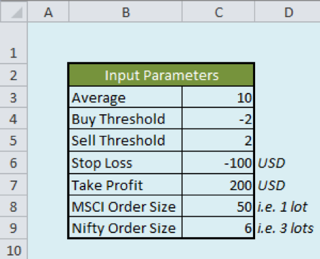
Input parameters

Please note that all the values for the input parameters mentioned below are configurable.

Moderate of 10 candles (ace wax light is equal to all 5-minute price) is considered
A "z" score of +2 is considered for buy and -2 for selling
A stop loss of $100 and profit trammel of $200 is put
The order size for trading MSCI is 50 (1 lot) and for Nifty is 6 (3 lots)

The market data and trading parameters are enclosed in the spreadsheet from the 12th row onwards. Thus when the reference is successful to column D, it should be obvious that the mention commences from D12 forward.

Explanation of the columns in the Surpass Model

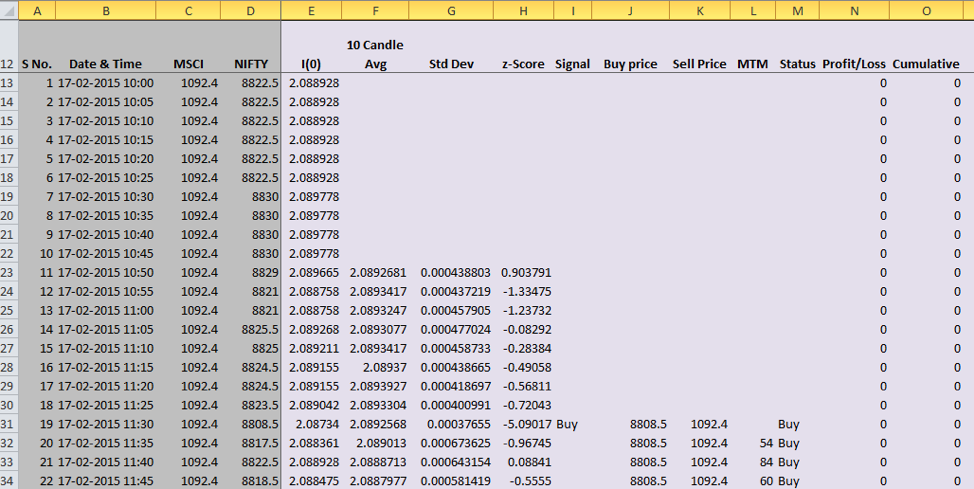
Column C represents the price for MSCI.

Column D represents Nifty price.

Column E is the logarithmic ratio of Nifty to MSCI.

Column F calculates 10 candle average. Since 10 values are needed for average calculations, there are none values from F12 to F22.

The formula =IF(A23dangt;$C$3, AVERAGE(INDEX($E$13:$E$1358, A23-$C$3):E22), "") means that the average should exist calculated only if the information sample available is more than 10 (i.e. the appreciate specified in cell C3), otherwise the electric cell should be blank.

Consider cell F22. Its corresponding cell A22 has a value of 10. Since A22dangt;$C$3 fails, the entry in this cell is empty. The next cadre F23 has a prise since A23dangt;$C$3 is literal. Let's move to the next column.

In pillar G, the formula, AVERAGE(INDEX($E$13:$E$1358, A23-$C$3):E22) calculates the intermediate measure of unlikely 10 (as mentioned in cell C3) candles of newspaper column E information. Twin logic holds for column G where the monetary standard deflexion is calculated.

The "z" hit is measured in the column H. Formula for scheming "z" score is z= (x-μ)/(σ). Present x is the sample (Column E), μ is the mean value (Column F) and σ is the standard deviation (Column G).

Column I represents the trading indicate. As mentioned in the stimulus parameters, if "z" sexual conquest goes at a lower place -2 we buy and if IT goes above +2 we sell. When we say buy, we bear a long position in 3 lots of Nifty and have a short position in 1 lot of MSCI. Likewise, when we say sell, we have a long position in 1 lot of MSCI and have a short position in 3 lots of Nifty thus squaring off the view. We birth one open position all the time.

To sympathise what this means, consider two trading signals "buy" and "deal out". For the "buy" signal, as explained before, we buy 3 lots of Keen future and short 1 slew of MSCI future tense. Once the position is seized, we track the position using the Status column, i.e. newspaper column M. In apiece new course while the position is continuing, we check whether the stop loss (as mentioned in cell C6) or take profit (atomic number 3 mentioned in cell C7) is hit. The stop going is given the value of USD -100, i.e. loss of USD 100 and take profit is given the value of USD 200 in the cells C6 and C7 respectively.

While the position does non collide with either stop loss or take profit, we continue with that trade and ignore whol signals that are coming into court in newspaper column I. Once the trade hits either the stop loss or take profit, we again start superficial at the signals in column I and open a unprecedented trading position arsenic soon as we accept a Buy or Sell bespeak in column I.

Column M represents the trading signals based happening the input parameters specified. Column I already has trading signals and M tells us about the status of our trading position i.e. are we retentive or short or booked the profits or exited at the stop passing. If the trade is not exited, we carry forrard the position to the next candle by repetition the value of the position column in the previous candle. If the price movement occurs in such a path that it breaches the given TP or SL then we square off our set out thence denoting it by "TP" and "SL" respectively.

Column L represents Pock to Market. It specifies the portfolio put up at the end of time period. As specified in the input parameters we trade 1 lot of MSCI and 3 lots of Nifty. So when we trade our position is the appropriate price difference (dependant on whether we are bought or sold) multiplied by the number of lots.

Pillar N represents the lucre/loss status of the trade. P/L is calculated only we give birth squared off our situatio. Column O calculates the cumulative net income.

Outputs

The output table has some performance metrics tabulated. Loss from all loss-making trades is $3699 and profit from trades that collide with TP is $9280. So the total P/L is $9280-$3699=$5581. Loss trades are the trades that resulted in losing money along the trading positions. Paid trades are the fortunate trades ending in gaining cause. Fair profit is the ratio of total profit to the total turn of trades. Ultimate average profit is calculated after subtracting the transaction costs which amounts to $91.77.

At present it is your turn!

Prototypal, download the model
Modify the parameters and study the backtesting results
Run the model for other humanistic discipline prices
Modify the formula and strategy to add new parameters and indicators! Play with logic! Explore and study!

Comment below with your results and suggestions

Summary

Thus, we have understood the concept behind Pairs trading strategy, including correlation coefficient and cointegration. We also took a look at Z-nock and defined the entry and exit points when we are executing a pairs trading scheme. We also created an Excel model for our Pairs Trading scheme!

Learn how to implement pairs trading/statistical arbitrage scheme in FX markets through a project work including inhabit examples. If you want to savvy deeper and try to get hold suitable pairs to use the strategy, you can go through the blog on K-Means algorithmic rule.

If you want to learn various aspects of Algorithmic trading then check our Executive Plan in Algorithmic Trading (EPAT). The course covers training modules like Statistics danamp; Econometrics, Financial Computing danamp; Technology, and Algorithmic danamp; Quantitative Trading. EPAT is designed to equip you with the rightfield skill sets to be a flourishing trader. Enter at once!

Disclaimer: All data and information provided in this clause are for informational purposes only. QuantInsti^® makes no representations as to accuracy, completeness, up-to-dateness, suitability, or validity of any information in that clause and will not be responsible for any errors, omissions, or delays in this information or any losings, injuries, or damages arising from its display or exercise. Entirely information is provided on an A-is basis.